
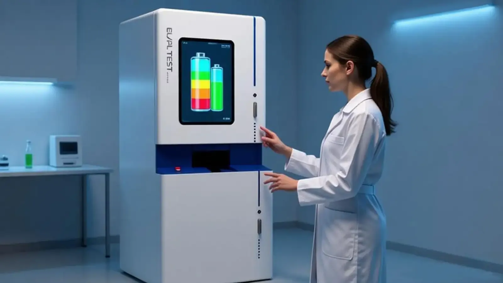
29 Defect Classes via AI Auto-Decision: From Feature Engineering to Deep Models
In 2017 PV EL defect identification still required 5–8 senior engineers to read images by hand. In 2025 our AI system labels 29 defect classes with confidence scores in 0.2 s. The path through took four algorithm generations — and each leap created new limits. This article doesn't dive into network architectures (plenty of academic papers do that). It walks through the engineering trade-offs of real production deployment.
1. Generation 1 (2017–2019): hand-crafted features + classical classifiers
The earliest pipeline was handcrafted features + SVM/Random Forest:
- Features: HOG, LBP, Gabor, GLCM
- Classifiers: one-vs-rest SVM (29 binary classifiers)
- Training data: 5,000 hand-labeled images
A classic engineering pain: 29 classes meant 29 binary classifiers; running them all took 1.2 s — unacceptable on a production line. Many factories ran only the top-5 frequent classes (microcracks, broken fingers, breakage, bad solder, low-efficiency) and human-sampled the other 24.
Gen 1 limitations:
- Feature engineering depended on engineer intuition; tuning cycle 2–4 weeks;
- Hand-crafted features brittle to brightness/angle changes;
- Accuracy ceiling ~85% — could not push higher;
- Adding a new defect class meant designing new features.
2. Generation 2 (2019–2021): end-to-end CNN classification
With ImageNet-era models maturing, we switched to ResNet50 end-to-end multi-class classification:
- Network: ResNet50 with multi-task heads (29-class label + defect location)
- Training data: 50K images
- Augmentation: random flip, brightness jitter, Cutout
- Inference: 0.15 s/image on a single V100
The Gen 2 leap was accuracy from 85% to 92%, and adding a new class meant data + fine-tune (no feature redesign). New problems emerged:
Gen 2 limitations:
- Severe class imbalance: microcracks 60% of samples, dislocations 1.2% — long-tail recall poor;
- Weak small-object detection: early ResNet recall on ~10 px defects only ~60%;
- No spatial-relation modeling: patterns like "microcrack + adjacent brightness drop" couldn't be explicitly leveraged.
3. Generation 3 (2021–2023): detection + segmentation + self-supervised pretraining
Two fundamental upgrades:
3.1 Dual-head architecture
- Detection head: YOLOv8 over 29 classes (bounding boxes)
- Segmentation head: U-Net per-pixel masks
- Shared backbone: EfficientNet-B4
Parallel heads pushed small-defect recall from 60% to 88% and gave customers "defect position + defect shape" simultaneously.
3.2 Self-supervised pretraining
PV images have unique textures (busbars, edges, cell tiling); generic ImageNet pretraining underperformed. We did MAE (Masked Autoencoder) self-supervised pretraining on 2M unlabeled PV images, then fine-tuned on 50K labeled.
Result:
- Accuracy: 92% → 96.5%
- Long-tail recall (dislocations, slip lines): 62% → 84%
- Inference: 0.15 s → 0.08 s (smaller but smarter backbone)
Gen 3 limitations:
- Model still large (85 M params) — edge deployment hard;
- No semantic understanding of defects — extrapolation to rare new classes weak;
- Cross-line / cross-factory generalization weak; new-factory deployment needed 200–500 local samples to fine-tune.
4. Generation 4 (2023–present): foundation models + vision-language alignment
The Gen 4 era borrows from foundation-model thinking:
4.1 Vision foundation model
Backbone replaced with DINOv2 / SAM — large (300M+ params) but generic representations. Engineering optimizations:
- Quantization: FP32 → INT8, model size 75 MB;
- Op fusion: Conv-BN-ReLU sequences fused → 2.3× faster;
- TensorRT deployment: 0.06 s/image on NVIDIA Jetson Orin.
4.2 Vision-language alignment
In partnership with the Nanjing Xiangning AI Institute, we encoded each defect's physical description (e.g., "microcrack: dark line caused by silicon-lattice fracture along stress lines, width 5–200 μm, mostly aligned with principal stress direction") via a CLIP-style approach. Outcome:
- A new defect class needs just 50–100 samples to reach 90% accuracy (vs 500+ before);
- The model can explain "why this class" via vision-language similarity;
- Cross-line generalization improves dramatically; new-factory sample need drops from 500 to 100.
4.3 Current numbers
| Metric | Gen 3 | Gen 4 |
|---|---|---|
| 29-class accuracy | 96.5% | 98.6% |
| Long-tail mAP | 0.72 | 0.86 |
| Edge inference | 0.08 s | 0.06 s |
| Model size | 320 MB | 75 MB (INT8) |
| New-factory samples needed | 500+ | 100+ |
5. Next gen (2025–2026): online continual learning
Gen 4 is still "train → freeze → deploy". Our 2026 direction is online continual learning — each customer line's model learns the line's specific patterns locally; newly discovered defect cases feed back into model weights. Challenges:
- Catastrophic forgetting: online learning can degrade old-task performance;
- Data privacy: customer-labeled data must not leave the line;
- Stability: line-model weights cannot drift on a single mislabel.
We're testing a federated + continual learning hybrid — local learning stays local; gradient aggregation goes to the central model securely. Targeted Q3 2026 grayscale deployment at 3–5 lighthouse customers.
6. Practical advice
"Which generation should I deploy?" — newer isn't always better:
- Tight cycle (<1s/wafer): Gen 3 or quantized Gen 4;
- Stable defect taxonomy: Gen 3 is sufficient and cheaper to deploy;
- Frequent new defect types: Gen 4 mandatory — generalization is the moat;
- Multi-line / multi-factory: Gen 4 + federated readiness.
EPL/PLEL/MC-W products ship with Gen 4 by default; existing customers receive algorithm upgrades free of charge.
For algorithm demos or a line-fit assessment, contact MVCreate at +86 159-5048-9233.
Originally published by Vision Potential (Nanjing MVCreate Intelligent Technology Co., Ltd.). Reproductions must credit the source.